Āryabhaṭa's Algorithmic Square Rooting
Learn How to Do Algorithmic Square Rooting from The Āryabhaṭiyam

So, the first thing to ask is - when did square rooting start and for what purpose? Since, my focus is Bhārat, the mention of square roots goes back all the way first in one of the śulba sūtras.
You may have heard about the Baudhayana Śulba Sūtra where a certain type of proof of the so-called Pythagoras theorem is given. Now, the purpose of these is of course practical and they are in fact, what Dr C K Raju calls, “manuals for masons.”
Nevertheless, the mathematics and the formulae should not be ignored as with our own epistemology, practical aspects of any subject are given high importance.
There are 7 known authors who wrote śulba sūtras and these are:
Baudhāyana
Āpastamba
Kātyāyana
Mānava
Maitrāyana
Vāraha
Vādhūla
Many of them have variations of the calculation of the diagonal, but the one we’re focusing on today would be Mānava, mainly because it goes as far as square rooting to get the exact value and is the first time, we encounter the term for square root.
Square is called Varga, root is called Mūla.
Square root, rather simply is Vargamūla.
In the Mānava śulba sūtra, section 10.1.3, 10th shloka, you’ll find
आयाममायामगुण विस्तारँ विस्तरेण तु ।
समस्य वर्गमूलँ यत् तत्कर्ण तद्विदो विदुः ॥
This talks about the square rooting of a diagonal (hypotenuse). I won’t elaborate on this as we’re going to go approximately a millenia forward after this to Āryabhaṭiyam where we find a square root algorithm, we can use even today.
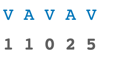
Before we get into it, we need to discuss the nomenclature of the Varga and Avarga positions. As you’re aware from above, varga is square, so varga position is a square position.
If we use a positional notation for places of the digits we can label every square place as a Varga and every non-square place as Avarga.
100 = 1 is squareable (1 x 1) therefore it is a Varga position
101 = 10 is not squareable therefore it is a Avarga position
102 = 100 is squareable (10 x 10) therefore it is a Varga position
103 = 1,000 is not squareable therefore it is a Avarga position
104 = 10,000 is squareable (100 x 100) therefore it is a Varga position
105 = 100,000 is not squareable therefore it is a Avarga position
And, so on and so forth.
We’ll use the labels V for Varga and A for Avarga.
Ok, let’s look at the algorithm now …
भागं हरेत् अवर्गात् नित्यं द्विगुणेन वर्गमूलेन ।
वर्गाद्वर्गे शुद्धे लब्धं स्थानान्तरे मूलं ॥
So, we’ll now address this step-by-step.
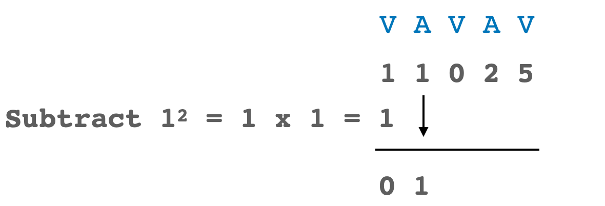
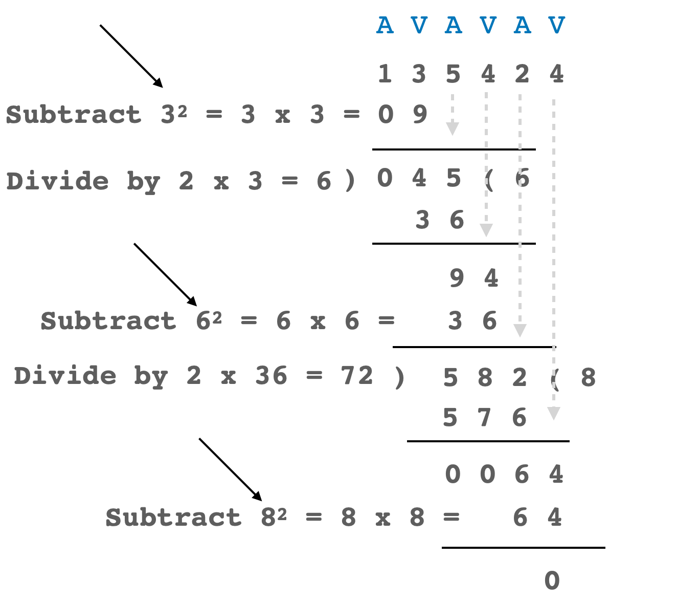
Let us take the number 11,025
Step 1 - Starting from the least significant digit (lowest place value), label the digits as varga or avarga. Then from the remaining (1 or 2) most significant digit(s), which constitutes varga-sthāna, subtract the square of the maximum number that is possible.
As you can see, we’ve labelled these as varga (square position) and avarga (non square position). The first we have to take the Varga position which will be either one or two digits. In this case it is a single digit of 1. The highest square we can subtract from this is 1.
Step 2 - The one thing you have to keep an eye on are the subtraction of the square numbers as they will become the part of the square root. You have to take twice the square root in each step. At the moment, we’ve only reached the solution of 1 and twice of 1 is one. You have to bring down the next digit and divide by twice the current square root obtained.
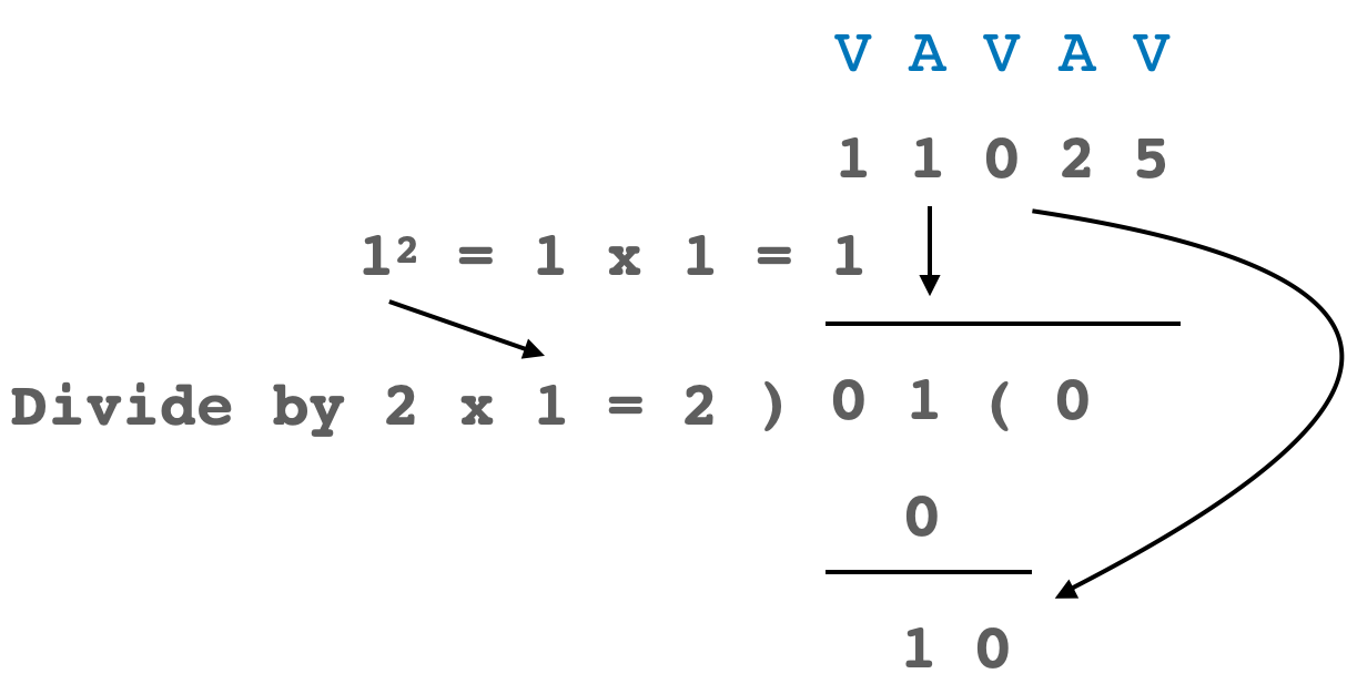
Note: Here we’re lucky as 2 is just bigger so we get zero. In the next step, we’re going to subtract the square of the quotient, so we have to ensure that this square of the quotient subtraction doesn’t create a negative number. There may be backtracking involved here and we may have to reduce the quotient to make this accommodation. That’s what makes this algorithmic.
Step 3 - Along with the remainder bring down the next digit in the varga place and subtract from it the square of the previous quotient. The square of the quotient here is the square of 0 which we can easily subtract from anything, so it’s a non-issue in this case.
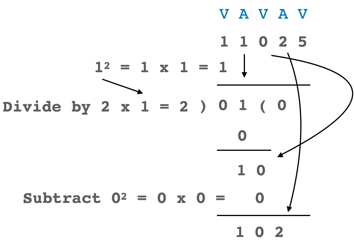
Then we pull down the next number. The square root obtained so far is 10 (It’s the square numbers that we’re subtracting. Now, we repeat the step of dividing by twice the obtained square root.
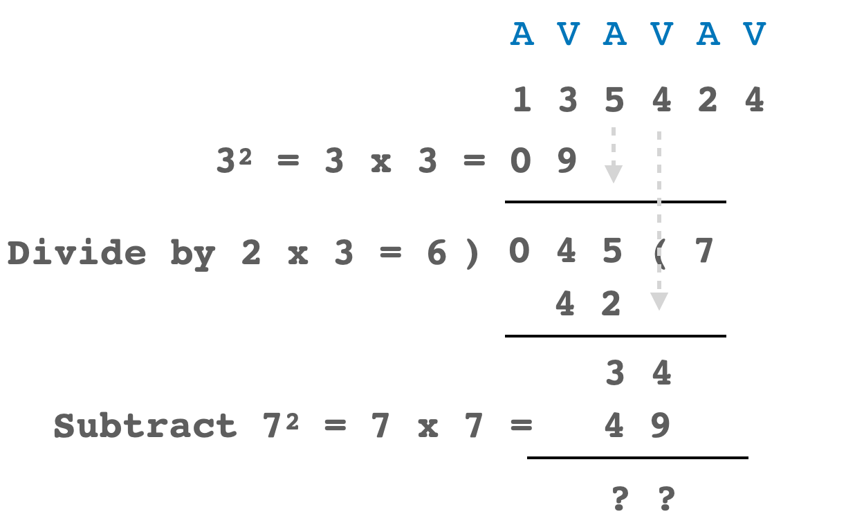
Let’s continue and finish all of the steps here.
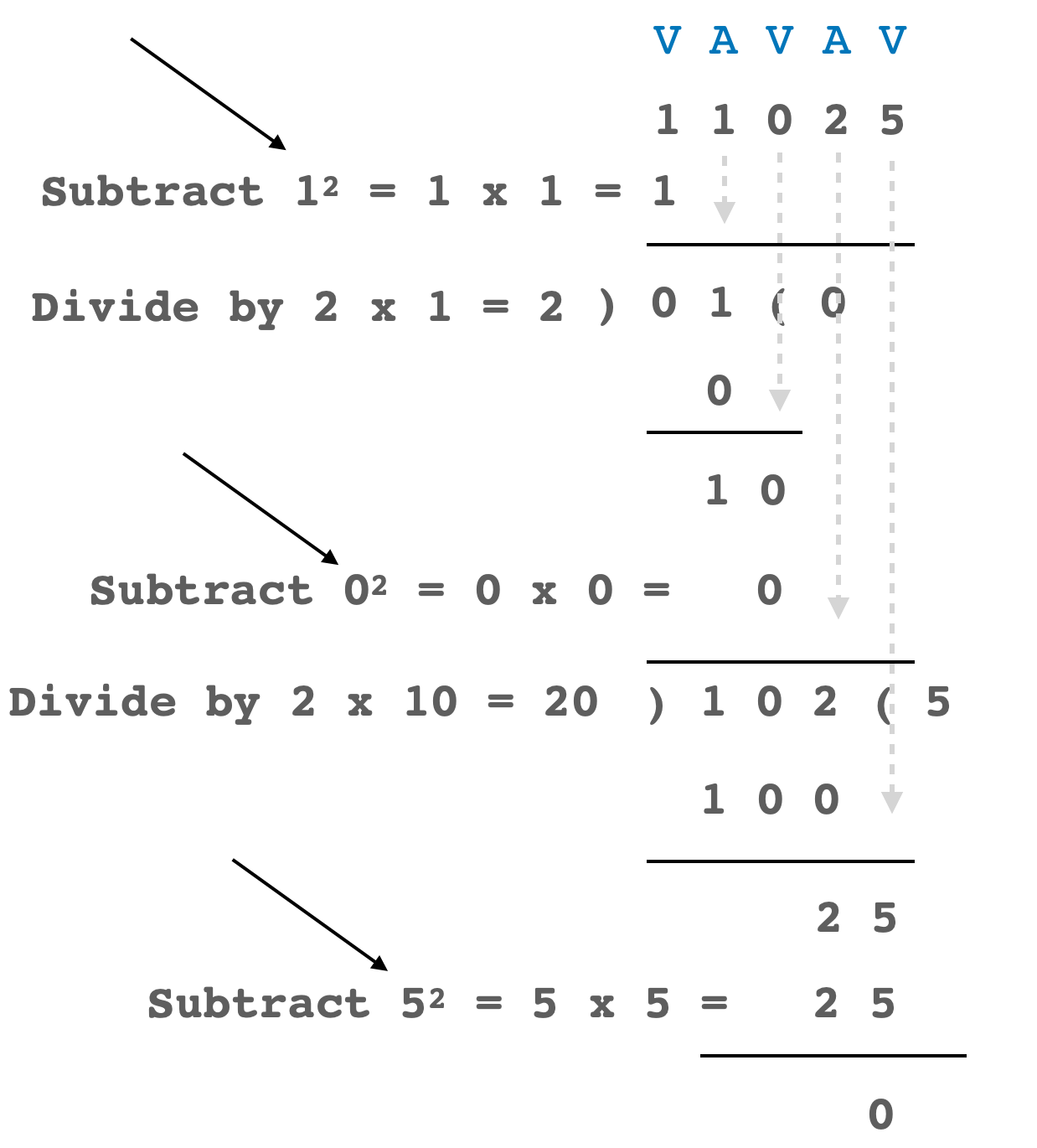
When we see the line of the square root obtained so far, it’s 105, and we can go no further, so that’s the answer. And, sure enough 105 x 105 = 11025.
Now, that we know the system, let’s explore these with some variations. The first of course would be the left most position being non-square or Avarga.
Here we have to take the first two digits. Otherwise, it’s pretty straight forward. The answer above comes to 621.
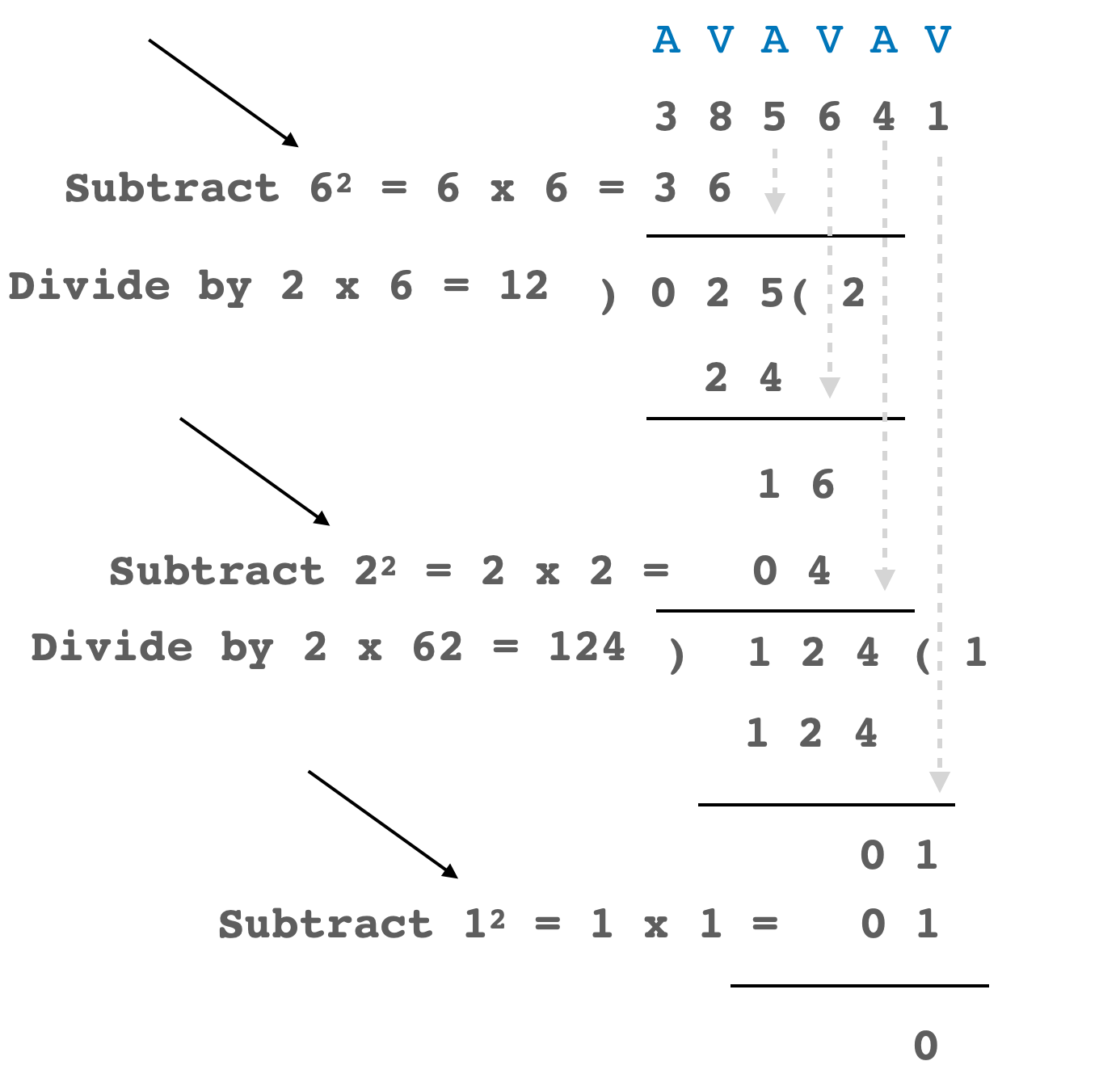
Now, in the next one, pay special attention to the first division step as shown below:
And the answer is 291.
Here, in the first division step we could have chosen to divide by 10 as 4 x 10 is 40. We could have even chosen 11 as 4 x 11 is still 44. There are two reasons we chose 9. The first is that we do not want to go beyond single digits on the square numbers. The second is that it would violate the rule of squares as in, if we took 11, the number to subtract from would be 0 + 6 = 6 and we would have to subtract 11 x 11 = 121 from it, making it negative. If we took 10, then we would have 46 and we would have to subtract 100 from it, again making it negative. So, the largest positive possibility is still 9 where we subtracted 81 from 86 letting us go to the next step.
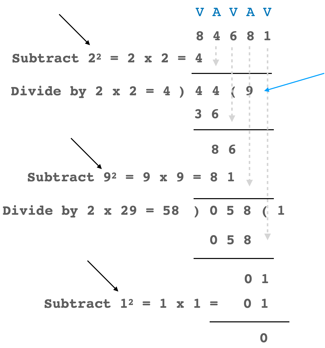
Now, let’s take one more example of backtracking to illustrate this.
So, we’re again getting a negative result which is a problem. We have to wait another 200 odd years for Brahmagupta’s rules for arithmetic to understand negative numbers. More on that another time.
So, we essentially backtrack by reducing the quotient by 1 from 7 to 6 and try again.
As you can see, now our routine works after one backtrack. The answer is 368.
What is interesting is the algorithmic nature of square rooting given so far back, at least a thousand years before the West was even aware of it. The algebraic roots in this are obvious.
A civilization has to have really evolved in their treatment of Mathematics before that can do something this advanced. The beauty is that we can even teach these to kids today.
There’s algorithmic cube rooting as well in this manuscript from Bhārat which dates back to the 4th/5th century CE. What’s also interesting is the mention of square roots at least a 1000 years prior to this in the Mānava Śulba Sūtra.
When you look at the Mathematics, it becomes rather obvious at how the scientific temperament of this land would have been.
Amazing to See This.. What a Treasure of Knowledge. WoW. Thank You